Section 5: Tree Methods & AVM Baseline
Learning Objectives
By the end of this section, students will be able to:
- Understand CART algorithm for regression trees
- Build random forest models for property valuation
- Analyze feature importance to identify key valuation drivers
- Evaluate tree-based models against linear baselines
- Implement production-candidate AVM using ensemble methods
PART 1: DECISION TREES AND INTERPRETABILITY
Decision trees offer something rare in machine learning: a model you can explain to anyone. Unlike the black-box nature of many algorithms, decision trees create a series of simple yes/no questions that mirror human reasoning. When a loan officer needs to justify why an application was denied, or a doctor needs to understand a diagnostic recommendation, the interpretability of decision trees becomes highly valuable.
The Logic of Recursive Partitioning
Decision trees learn by recursively splitting data into increasingly homogeneous groups. Starting with all data at the root node, the algorithm searches for the single feature and threshold that best separates the classes. This process repeats for each resulting subset until stopping criteria are met. The result is a hierarchical structure where each path from root to leaf represents a decision rule.
Each node represents a decision point in the tree. The root node contains all training data. Internal nodes apply decision rules to split data. Leaf nodes contain final predictions and stop further splitting.
A split is a decision rule that divides data at a node. Each split asks: “Is feature X ≤ threshold value?” The algorithm tests every possible feature and threshold combination to find the split that best separates the classes.
Think of it like playing twenty questions. Each question narrows down the possibilities until you reach a specific answer. The algorithm automatically discovers which questions to ask and in what order and optimizes for the purest possible groups at each step.
Example: Credit card fraud detection. A credit card company wants to predict fraud. The decision tree starts by asking: “Is the transaction amount over $500?” If yes, it then asks: “Is it at a merchant the customer has never used?” If yes again: “Is it more than 100 miles from the last transaction?” After just three questions, the tree identifies transactions with a 78% fraud probability. The path is transparent: large amount + new merchant + distant location = high risk. Every stakeholder understands this logic without needing statistics training.
Experience how decision trees create rectangular decision regions by clicking to add splits:
What to observe: - Each click adds a vertical or horizontal split - Regions become more homogeneous (lower Gini impurity) with each split - The algorithm naturally creates rectangular decision boundaries - Hover over regions to see their purity scores
The beauty lies in the simplicity. Each split considers only one feature at a time and creates axis-aligned decision boundaries that partition the feature space into rectangular regions. While this limits flexibility compared to other algorithms, it produces rules that humans naturally understand.
Measuring Impurity: Gini vs Entropy
The algorithm needs a way to measure impurity - how mixed or disordered each group is. Pure nodes contain samples from only one class (impurity = 0). Maximum impurity occurs when classes are perfectly balanced.
Two main metrics dominate: Gini impurity and entropy. Both quantify the disorder in a node, reaching minimum (0) when all samples belong to the same class and maximum when classes are perfectly balanced.
Gini = 1 - Σ(p_i)²
Where:
- p_i = proportion of samples belonging to class i
- Ranges from 0 (pure) to 0.5 (maximum impurity for binary)
- Used by CART algorithm
Entropy = -Σ(p_i × log₂(p_i))
Where:
- p_i = proportion of samples belonging to class i
- Ranges from 0 (pure) to 1 (maximum impurity for binary)
- Used by ID3 and C4.5 algorithms
Which metric should you choose? In practice, they produce very similar trees. Gini is computationally faster (no logarithms) and has become the default in most implementations. Entropy has theoretical connections to information theory but requires slightly more computation. The choice rarely impacts final model performance significantly.
The algorithm evaluates every possible split on every feature and calculates the weighted average impurity of the resulting child nodes. The split that achieves the largest impurity reduction (also called information gain) is selected. This greedy algorithm chooses the best split at each step without looking ahead. Why not consider all possible tree structures? The computational cost would be astronomical. Instead, the algorithm makes locally optimal decisions at each node, accepting that this approach might miss globally optimal solutions. This trade-off between computational efficiency and optimality works well in practice, producing trees that generalize effectively while remaining interpretable.
Growing Trees: When to Stop
Left unchecked, a decision tree will grow until every leaf contains exactly one sample, achieving perfect training accuracy but terrible generalization. Several parameters control tree growth:
Maximum depth limits how many levels the tree can have. Shallow trees (depth 3-5) create simple, interpretable models but might underfit. Deep trees capture complex patterns but risk overfitting and lose interpretability.
Minimum samples per split prevents creating nodes with too few samples. Requiring at least 20 samples to split forces the tree to make decisions based on meaningful patterns rather than noise.
Minimum samples per leaf guarantees each prediction is based on sufficient evidence. A leaf with only one sample memorizes that specific case rather than learning a pattern.
from sklearn.tree import DecisionTreeClassifier
from sklearn.model_selection import cross_val_score

# Compare different tree depths
depths = [3, 5, 7, 10, None]  # None means no limit
for depth in depths:
    tree = DecisionTreeClassifier(
        max_depth=depth,
        min_samples_split=20,
        min_samples_leaf=10,
        random_state=42
    )
    scores = cross_val_score(tree, X_train, y_train, cv=5)
    print(f"Depth {depth}: CV Score = {scores.mean():.3f} (+/- {scores.std():.3f})")
These pre-pruning techniques prevent overfitting by stopping growth early. However, they might miss important patterns that only emerge deeper in the tree. This motivates post-pruning approaches that first grow a complex tree and then simplify it.
Cost-Complexity Pruning: Finding the Right Size
Cost-complexity pruning (also called minimal cost-complexity pruning) provides a principled way to simplify trees after they’re fully grown. The technique balances accuracy against tree complexity using a parameter α (alpha) that penalizes each additional leaf node.
R_α(T) = R(T) + α × |T|
Where:
- R(T) = misclassification rate of tree T
- |T| = number of leaf nodes
- α = complexity parameter (higher values favor simpler trees)
The algorithm identifies the sequence of nested subtrees that minimize this cost-complexity measure for increasing values of α. When α = 0, the full tree is optimal. As α increases, simpler trees become preferable, until eventually a single-node tree (predicting the majority class) minimizes the measure.
from sklearn.tree import DecisionTreeClassifier
import matplotlib.pyplot as plt

# Get the pruning path
clf = DecisionTreeClassifier(random_state=42)
path = clf.cost_complexity_pruning_path(X_train, y_train)
ccp_alphas, impurities = path.ccp_alphas, path.impurities

# Train trees with different alpha values
trees = []
for ccp_alpha in ccp_alphas:
    tree = DecisionTreeClassifier(random_state=42, ccp_alpha=ccp_alpha)
    tree.fit(X_train, y_train)
    trees.append(tree)

# Find best alpha via validation
train_scores = [tree.score(X_train, y_train) for tree in trees]
test_scores = [tree.score(X_test, y_test) for tree in trees]

# The optimal alpha balances training and test performance
best_idx = np.argmax(test_scores)
best_alpha = ccp_alphas[best_idx]
print(f"Best alpha: {best_alpha:.4f}")
Cross-validation helps select the optimal α value. The pruned tree often achieves similar or better test accuracy with far fewer nodes, improving both interpretability and generalization.
Feature Importance: Understanding What Matters
Decision trees naturally provide feature importance scores that quantify each variable’s contribution to reducing impurity. Features used near the root have high importance since they partition the most data. Features never selected have zero importance.
Example: Hospital readmission risk prediction. A hospital predicts 30-day readmission risk using 50 patient variables. The decision tree’s feature importance reveals that just five variables drive most predictions: number of previous admissions (0.31), discharge medication count (0.22), age (0.18), primary diagnosis category (0.12), and insurance type (0.08). The remaining 45 features contribute less than 10% combined. This insight helps administrators focus on the factors that truly matter for intervention programs.
Feature importance helps with feature selection, identifying which variables to collect in production systems, and providing business insights about what drives outcomes. However, importance scores can be unstable, changing significantly with different random seeds or slight data variations.
Visual Interpretation: Seeing the Logic
One of decision trees’ greatest strengths is visualization. The tree structure can be plotted to show the exact decision process:
Explore a complete decision tree for loan approval decisions. Click nodes to inspect details, hover to highlight decision paths, and use the depth slider to see pruning effects:
| Aspect | Decision Trees | Black-Box Models |
|---|---|---|
| Explainability | Every prediction traceable | Difficult to explain individual predictions |
| Feature relationships | Only captures interactions explicitly | Can model complex interactions implicitly |
| Regulatory compliance | Easy documentation and auditing | Requires additional explanation techniques |
| Debugging | Can inspect specific decision paths | Limited visibility into failures |
| Trust building | Stakeholders understand the logic | Requires faith in the algorithm |
Handling Different Data Types
Decision trees elegantly handle both numerical and categorical features without preprocessing. For numerical features, the algorithm considers all possible thresholds between adjacent values. For categorical features with k categories, it evaluates all 2^(k-1) - 1 possible binary partitions (though many implementations use approximations for efficiency).
Missing values present interesting opportunities. Rather than requiring imputation, some implementations use surrogate splits. When the primary split variable is missing, the algorithm uses another variable that produces similar partitions. This approach maintains the tree’s interpretability while handling real-world data messiness.
The algorithm treats each feature independently at each split, which means it naturally performs feature selection. Irrelevant features simply won’t be chosen for splits. This differs from linear models where irrelevant features still receive coefficients, even if small ones.
Limitations and Failure Modes
Despite their advantages, decision trees have significant limitations. They create axis-aligned decision boundaries, struggling with diagonal or curved patterns. A linear relationship might require many splits to approximate, creating an unnecessarily complex tree.
Trees are also notoriously unstable. Small changes in training data can produce completely different trees with similar performance but different structures. This instability makes single trees unsuitable when consistency matters.
The greedy splitting strategy can miss optimal solutions. Sometimes accepting a suboptimal split early enables much better splits later, but the algorithm can’t look ahead to discover these opportunities. This motivates ensemble methods like random forests that combine many trees to overcome individual weaknesses.
Example: Customer churn prediction instability. A marketing team uses a decision tree to predict customer churn. The tree achieves 85% accuracy, identifying that customers who haven’t logged in for 30 days and have declined usage over three months are likely to churn. However, when retrained monthly, the tree structure changes dramatically even though performance remains stable. One month “declined usage” is the root split; the next month it’s “days since login.” This instability makes it hard to derive consistent business rules or track how decision factors evolve over time.
Regression Trees: Predicting Continuous Values
While the focus has been on classification, decision trees also handle regression by predicting continuous values. Instead of class probabilities, each leaf contains the mean target value of its training samples. Instead of Gini or entropy, the algorithm minimizes the sum of squared residuals or mean absolute error.
Regression trees partition the feature space into rectangles, predicting a constant value within each region. This creates a piecewise constant approximation that can model non-linear relationships but produces discontinuous predictions. The tree can’t extrapolate beyond the range of training data, always predicting values between the minimum and maximum observed targets.
Practical Implementation Guidelines
Start with a relatively shallow tree (max_depth=3-5) to establish a baseline and understand the primary decision factors. Visualize this simple tree to verify it makes intuitive sense. Then systematically increase complexity, monitoring validation performance to find the sweet spot between underfitting and overfitting.
Use cost-complexity pruning when you need a principled approach to tree simplification. The pruning path reveals how performance degrades as the tree simplifies, helping you choose an appropriate trade-off between accuracy and interpretability.
For imbalanced datasets, adjust the class_weight parameter or use balanced splitting criteria. Trees naturally favor majority classes, so explicit balancing guarantees minority classes get appropriate attention in splits.
Consider ensemble methods when pure performance matters more than interpretability. Random forests and gradient boosting overcome single trees’ instability and limited flexibility while sacrificing the ability to trace individual predictions.
Monitor feature importance stability across different random seeds and data samples. Stable important features represent reliable patterns, while unstable ones might indicate noise or multicollinearity. Use this information to guide feature engineering and data collection efforts.
Interpretability is decision trees’ superpower. When stakeholders need to understand and trust model decisions, when regulations require explainable AI, or when you need to discover business rules from data, decision trees offer unmatched transparency. They might not achieve state-of-the-art performance, but they provide something often more valuable: understanding.
PART 2: BAGGING METHODS
Learning Objectives
By the end of this section, you will:
- Understand bootstrap aggregation mechanics and variance reduction principles
- Implement random forests with feature subsampling for improved diversity
- Use out-of-bag error estimation for model validation without separate test sets
- Tune hyperparameters to optimize random forest performance
- Recognize when bagging helps versus hurts different model types
- Apply parallel training strategies for computational efficiency
The Single Model Problem
You train a decision tree on your customer churn data and it makes confident predictions. But what happens when you rerun the model after adding this week’s new customer records? The tree structure shifts completely—splits that appeared at the top move down or disappear, and features that seemed unimportant now drive decisions. This behavior reveals high variance: small changes in training data produce large changes in the model. A single tree tells you as much about which samples you happened to include as it does about the actual churn pattern.
Bootstrap aggregation addresses this problem through a counterintuitive solution: you train many unstable models on slightly different data, then average their predictions. This ensemble approach, known as bagging, transforms variance from a weakness into a strength.
Bootstrap Aggregation Mechanics
Bagging begins with resampling. You take your training data and create multiple bootstrap samples by randomly drawing observations with replacement. Each bootstrap sample has roughly 63% unique observations from the original data (the remaining 37% are duplicates or were never selected). This resampling injects controlled randomness into the training process.
You train a separate model on each bootstrap sample. For regression problems, the bagged prediction averages predictions across all models. For classification, you use majority voting: count the predicted class from each model and select the most frequent. Some implementations use soft voting (averaging predicted probabilities) when base models provide probability estimates.
Example: Real estate bagging ensemble. Think about some of the real estate projects we built in previous lectures—those regression models predicting home prices from square footage, location, and age. Now you build 100 regression trees on bootstrap samples of recent home sales. One tree over-weights square footage because its sample contained unusual mansions (five properties over 8,000 square feet that distorted the pattern). Another under-weights location due to sampling bias toward suburban homes. When you average these 100 predictions, the individual biases partially cancel out. The mansion-heavy tree pulls prices up while the suburban-focused tree pulls them down, and the averaged prediction settles closer to the true relationship than any single tree provides.
Watch how bootstrap sampling creates diverse training sets. Click “Generate Bootstrap Samples” to see how drawing with replacement produces samples with ~63% unique observations and duplicates:
Variance Reduction Through Averaging
The statistical foundation for bagging rests on variance reduction. When you average predictions from multiple models, random errors tend to cancel out while systematic patterns reinforce each other. In practice, predictions from bootstrap samples are positively correlated (they share about 63% of training data), which limits but does not eliminate the variance reduction.
Prediction error comes from three sources: bias (systematic mistakes from model assumptions), variance (sensitivity to training data changes), and irreducible noise. Bagging primarily targets the variance term. Each bootstrap sample produces a slightly different model, and these differences stem from sampling variation rather than fundamental model capacity. When you average across samples, this smooths these fluctuations without substantially increasing bias.
This variance reduction works best for high-variance learners like deep decision trees or nearest neighbor models with small k. These algorithms are sensitive to small training set changes. A high-variance model responds to data like a Formula 1 car responds to road conditions: every bump, temperature change, or surface texture alters handling significantly. Low-variance models like linear regression behave like a heavy truck: they maintain steady performance across bootstrap samples because their coefficient estimates barely shift. When you bag a stable model, it returns predictions nearly identical to the original. You spend 100 times the computational cost to get a 1% improvement, which rarely makes sense in production.
Bagging provides implicit regularization without explicit penalties. A single deep tree memorizes training data noise and achieves near-perfect training accuracy but poor test performance. When you average 100 such trees trained on different bootstrap samples, the memorized noise differs across trees (one tree memorizes patient #47’s unusual values, another memorizes patient #83’s). These memorization errors cancel out when averaged, while true patterns that appear consistently across samples remain. This differs from explicit regularization (like Lasso) that constrains model parameters directly.
Random Forests and Feature Subsampling
You implement bagging on your classification problem and performance improves, but not as much as you expected. When you inspect the first few splits across your 100 trees, you find they nearly all split on the same three features in the same order. The trees remain highly correlated because bootstrap sampling alone does not force them to explore different feature combinations. Averaging correlated predictions provides less variance reduction than averaging diverse predictions.
Random forests address this limitation and have become the default choice for tree-based ensembles. The method adds feature subsampling to bagging: at each split in each tree, the algorithm considers only m features that it randomly selects from the full set of p predictors. This parameter, commonly called max_features or mtry, introduces decorrelation between trees.
How the Algorithm Works
The random forest training process adds one constraint to standard bagging. You still create B bootstrap samples and train one tree on each sample, but now each split point in each tree operates under a feature budget. When the algorithm evaluates where to split a node, it randomly selects m features from all p available features, then finds the best split using only those m candidates. The next node in the same tree gets a different random subset of m features.
This feature subsampling happens at every single split. A tree might consider features [1, 5, 12, 20] at the root node, features [3, 8, 15, 22] at the left child, and features [2, 9, 14, 19] at the right child. No feature gets special treatment. Even the strongest predictor might not appear in the candidate set for a particular split, which forces the tree to explore alternative patterns.
Watch how random forests select different feature subsets at each split. Click “Next Split” to see how m = 4 features are randomly chosen from p = 12 total features, creating tree diversity:
Example: Credit risk feature subsampling. Consider a credit risk model with 60 features where debt-to-income ratio predicts default most strongly. Without feature subsampling, 95 of your 100 trees split on debt-to-income ratio at the root. With random forests using m = √60 ≈ 8, only about 13 trees (8/60 × 100) have debt-to-income ratio available at the root split. The remaining 87 trees discover different patterns through features like payment history, credit utilization, or employment stability.
Choosing the Feature Subset Size
The m parameter controls the bias-variance tradeoff within the ensemble. Smaller m values increase tree diversity (lower correlation) but force trees to use suboptimal splits more often (higher individual tree error). Larger m values let trees find better splits but make trees more similar. The defaults balance these competing forces:
| Problem Type | Default m | Rationale |
|---|---|---|
| Classification | √p | Moderate decorrelation for categorical outcomes |
| Regression | p/3 | Stronger decorrelation needed for continuous targets |
When you set m = p, this recovers standard bagging without any feature randomization. When you set m = 1, every split uses a randomly chosen single feature, which creates extremely diverse but weak trees. Research shows the defaults work well across most problems, though you should tune m when features have vastly different predictive strengths or when you suspect high correlation among predictors.
from sklearn.ensemble import RandomForestClassifier, RandomForestRegressor

# Classification with default m = sqrt(p)
rf_classifier = RandomForestClassifier(
    n_estimators=100,
    max_features='sqrt',  # ~sqrt(n_features)
    random_state=42
)

# Regression with default m = p/3
rf_regressor = RandomForestRegressor(
    n_estimators=100,
    max_features=0.33,  # p/3
    random_state=42
)

# Custom feature subset for high-dimensional data
rf_custom = RandomForestClassifier(
    n_estimators=100,
    max_features=10,  # Fixed number of features
    random_state=42
)
Out-of-Bag Error Estimation
Each bootstrap sample leaves out roughly 37% of training observations. These out-of-bag (OOB) samples provide a built-in validation set. For each observation, you collect predictions from all trees that did not see that observation during training, then average those predictions. The OOB error compares these predictions against true values across all observations.
The OOB error estimate approximates test set performance without requiring a separate holdout set. This is particularly valuable when training data is limited. However, research shows OOB error can overestimate true prediction error in certain settings: balanced binary classification, small sample sizes, many predictors with weak correlations, or large feature subset sizes.
Build a random forest and select different trees to see which samples are in-bag (blue) vs out-of-bag (yellow). Notice how each tree uses different OOB samples for validation:
from sklearn.ensemble import RandomForestClassifier

# Enable OOB scoring
rf = RandomForestClassifier(
    n_estimators=100,
    oob_score=True,
    random_state=42
)
rf.fit(X_train, y_train)

# OOB error approximates test error
oob_accuracy = rf.oob_score_
oob_error = 1 - oob_accuracy
OOB error estimation works only for bagging-based methods. Boosting and other sequential ensemble methods cannot use OOB error because each model depends on previous models’ predictions, which breaks the independence assumption.
Cross-Validation vs OOB Error
Do you still need cross-validation when using OOB error? Yes, for hyperparameter tuning. OOB error estimates performance for a specific model configuration, but when you compare OOB scores across different max_features or max_depth values, this introduces selection bias. Use cross-validation to tune hyperparameters, then use OOB error to monitor performance during training or when adding more trees.
Think of OOB as a fast approximation for a single model, cross-validation as the rigorous method for comparing multiple configurations. A marketing model uses 5-fold CV to choose between m = √p and m = p/3 (takes 45 minutes), then uses OOB error to track whether adding trees beyond 200 improves performance (takes 2 minutes). This hybrid approach balances rigor with computational efficiency.
Selecting the Number of Trees
How many trees should you train? Performance improves rapidly from B = 10 to B = 100, then plateaus. Most practitioners default to B = 100 for prototyping and B = 500 for production models. Plot OOB error against number of trees: when the error curve flattens (changes less than 0.001 for 50 additional trees), adding more trees wastes computation.
Example: Tree count optimization. A customer segmentation model reaches stable performance at B = 150. Training 500 trees improves accuracy by 0.002 but triples training time from 12 to 38 minutes. The marginal benefit of additional trees diminishes because averaging already captures the main patterns. Unlike some algorithms where more capacity always helps, bagging shows clear convergence where extra trees provide minimal gains.
from sklearn.ensemble import BaggingRegressor
from sklearn.tree import DecisionTreeRegressor

# Start with 100 trees for development
bagged_trees = BaggingRegressor(
    estimator=DecisionTreeRegressor(max_depth=None),
    n_estimators=100,
    random_state=42
)

# Scale to 500 trees for production
production_model = BaggingRegressor(
    estimator=DecisionTreeRegressor(max_depth=None),
    n_estimators=500,
    random_state=42,
    n_jobs=-1  # Use all CPU cores
)
Tuning Random Forest Hyperparameters
Now that you understand validation methods, you can systematically optimize random forest performance. Random forests require fewer tuning decisions than most algorithms, but several parameters affect performance substantially. Which parameters matter most when you face a new dataset? The answer depends on your data characteristics and computational budget.
Tree complexity parameters control how deep and detailed each tree becomes. max_depth limits how many splits each tree makes. Unrestricted depth (the default) works well because averaging reduces overfitting, but set max_depth=20 when training time becomes a constraint. You can also control complexity through leaf constraints: min_samples_leaf sets the minimum observations at terminal nodes (prevents tiny leaves that memorize noise), while max_leaf_nodes directly limits total leaves (alternative to depth limits that some practitioners find more intuitive).
Split control parameters determine when nodes divide. min_samples_split sets the minimum observations needed before attempting a split. The default of 2 works for most cases, but increase to 10 or 20 when you have noisy data or thousands of observations. Pair this with min_samples_leaf for balanced control: a node with 20 observations and min_samples_split=10 can split, but only if each child gets at least min_samples_leaf observations.
The bootstrap parameter controls whether trees train on bootstrap samples (random sampling with replacement) or the full dataset. Setting bootstrap=True (the default) defines bagging. Setting it to False creates a different ensemble method called pasting, where each tree sees the entire dataset but different feature subsets still provide diversity through max_features.
| Parameter | Purpose | Default | When to Tune |
|---|---|---|---|
max_depth |
Limits tree depth | None | Large datasets, long training times |
min_samples_split |
Min samples to split node | 2 | Noisy data, prevent overfitting |
min_samples_leaf |
Min samples at leaf | 1 | Smooth predictions, reduce noise sensitivity |
max_leaf_nodes |
Total leaf limit | None | Intuitive complexity control |
bootstrap |
Use bootstrap sampling | True | Rarely changed (defines bagging) |
Example: Fraud detection hyperparameter configuration. A fraud detection model with 50,000 transactions uses these settings:
max_features='sqrt',max_depth=25,min_samples_split=20,min_samples_leaf=10. This balances accuracy (0.94 AUC) against training time (8 minutes on 4 cores). Removing depth restrictions improves AUC to 0.95 but training takes 45 minutes. Themin_samples_leafconstraint prevents the model from creating leaves with fewer than 10 transactions, which would likely represent fraudulent patterns specific to individual accounts rather than generalizable fraud signals.
from sklearn.ensemble import RandomForestClassifier
from sklearn.model_selection import GridSearchCV

# Define parameter grid
param_grid = {
    'n_estimators': [100, 200, 500],
    'max_features': ['sqrt', 'log2', 10],
    'max_depth': [None, 20, 30],
    'min_samples_split': [2, 10, 20],
    'min_samples_leaf': [1, 5, 10],
    'max_leaf_nodes': [None, 50, 100]
}

# Grid search with cross-validation
rf = RandomForestClassifier(random_state=42, bootstrap=True)
grid_search = GridSearchCV(
    rf,
    param_grid,
    cv=5,
    scoring='roc_auc',
    n_jobs=-1
)
grid_search.fit(X_train, y_train)

# Best configuration
best_params = grid_search.best_params_
The class weight parameter handles imbalanced datasets. Set class_weight='balanced' to automatically adjust for class imbalance, or class_weight='balanced_subsample' to balance each bootstrap sample separately. For regression, max_samples controls bootstrap sample size: values less than 1.0 create smaller samples, which increases diversity but may underfit.
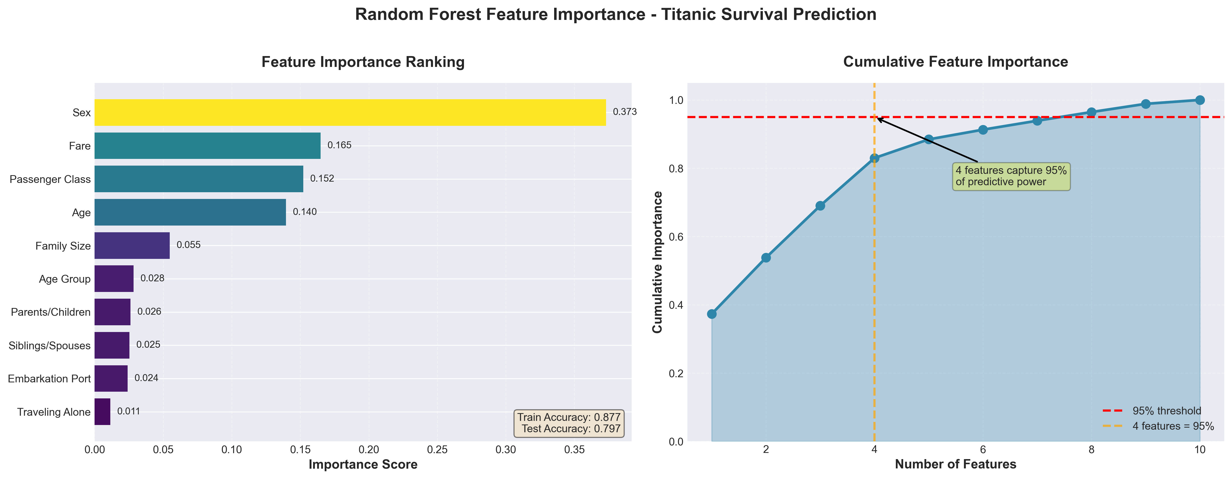
Feature Importance from Random Splits
After training and tuning your random forest, feature importance analysis reveals which predictors drive model decisions. Random forests provide a natural feature importance metric that aggregates information across all trees. For each feature, the algorithm measures how much each split using that feature improves prediction accuracy (measured by Gini impurity reduction for classification or variance reduction for regression), then averages these improvements across all trees where the feature appeared.
Features that appear in many splits and produce large improvements receive high importance scores. Features that rarely split nodes or produce small improvements when they do split receive low scores. This metric helps identify which predictors drive your model, though it can overweight continuous features or high-cardinality categorical features that offer more split opportunities.
# Train random forest and extract feature importance
rf = RandomForestClassifier(n_estimators=100, random_state=42)
rf.fit(X_train, y_train)

# Get importance scores
importance_scores = rf.feature_importances_
feature_names = X_train.columns

# Sort features by importance
import pandas as pd
importance_df = pd.DataFrame({
    'feature': feature_names,
    'importance': importance_scores
}).sort_values('importance', ascending=False)
Feature importance scores sum to 1.0 across all features. A feature with importance 0.15 contributes roughly 15% of the model’s total predictive ability, though this interpretation requires care because features often correlate with each other.
Parallel Training Advantages
Bagging offers a significant computational benefit: each bootstrap sample and each tree can train independently. Unlike boosting (covered in Section 7), where each model must wait for the previous model to finish, bagging models have no dependencies. This enables parallel processing across multiple CPU cores or distributed systems.
When you train 100 decision trees in sequence, this takes 100 times longer than training one tree. When you train 100 trees in parallel on 10 cores, this takes roughly 10 times longer than one tree, assuming load balancing and minimal overhead. For large datasets or complex base learners, this parallelization makes bagging computationally feasible.
Most implementations default to using all available CPU cores. The n_jobs=-1 parameter in scikit-learn splits model training across cores automatically. For random forests with hundreds of trees, this parallel training reduces wall-clock time substantially.
from sklearn.ensemble import RandomForestClassifier

# Single core training (slow)
rf_single = RandomForestClassifier(
    n_estimators=500,
    n_jobs=1,
    random_state=42
)

# All cores training (fast)
rf_parallel = RandomForestClassifier(
    n_estimators=500,
    n_jobs=-1,  # Use all available cores
    random_state=42
)
The independence of training also simplifies distributed computing. Each worker node can build its assigned trees using its subset of data and communicate only final model parameters back to the coordinator. This pattern scales well to cluster computing frameworks.
When Bagging Helps vs Hurts
High-variance models: Decision trees with no depth limit, neural networks with high capacity, and k-nearest neighbors with small k benefit substantially from bagging. These models overfit individual training sets but capture different aspects of the underlying pattern. Averaging reduces overfitting while preserving flexibility.
Stable, low-variance models: Linear regression, logistic regression, and other parametric models produce similar predictions across bootstrap samples. The averaged prediction nearly equals the single-model prediction but costs B times more computation. Bagging stable models slightly increases bias without sufficient variance reduction to justify the expense.
Small training sets: With hundreds of observations, bootstrap samples vary substantially and bagging provides clear benefits. Medical diagnosis models with 300 patient records or fraud detection with 400 labeled cases see meaningful accuracy gains. With thousands of observations, bootstrap samples differ only slightly from each other. Variance reduction still occurs but becomes less pronounced.
Class imbalance: Random forests handle imbalanced classes better than single trees but still struggle when one class appears 100 times more often than another. Bootstrap sampling maintains the original class distribution, which means rare classes get few training examples per tree. Set class_weight='balanced' to automatically adjust for imbalance, or use class_weight='balanced_subsample' to balance each bootstrap sample separately. A churn model with 5% positive cases improves recall from 0.42 to 0.68 with balanced class weights.
Interpretability tradeoff: A single decision tree clearly shows which features drive predictions and how they interact. A forest of 100 trees obscures these relationships. Feature importance metrics help but the model becomes harder to explain to stakeholders. Choose bagging when prediction accuracy matters more than interpretation.
Model correlation: Bagging works less effectively when base models already make similar predictions. If every tree splits on the same features in the same way, averaging provides little benefit. This correlation problem motivated feature subsampling in random forests. If correlation persists even with feature subsampling, other ensemble methods like boosting may work better.
Example: Customer lifetime value prediction comparison. A marketing team predicts customer lifetime value using 500 customers with 30 behavioral features. A single regression tree achieves RMSE of $850. Bagged trees reduce RMSE to $620 (27% improvement). Linear regression achieves $720 alone and $715 with bagging (minimal improvement). The high-variance tree model benefits; the low-variance linear model does not.
References
Breiman, L., Friedman, J., Stone, C. J., & Olshen, R. A. (1984). Classification and regression trees. CRC Press. https://www.taylorfrancis.com/books/mono/10.1201/9781315139470/classification-regression-trees-leo-breiman
Hastie, T., Tibshirani, R., & Friedman, J. (2009). Tree-based methods. In The elements of statistical learning (2nd ed., pp. 305-317). Springer. https://hastie.su.domains/ElemStatLearn/
Quinlan, J. R. (1986). Induction of decision trees. Machine Learning, 1(1), 81-106. https://link.springer.com/article/10.1007/BF00116251
Louppe, G. (2014). Understanding random forests: From theory to practice. arXiv preprint. https://arxiv.org/abs/1407.7502
Frenzel, T. (2023). KB Ensemble Learning — Part 1. Medium. https://prof-frenzel.medium.com/kb-ensemble-learning-part-1-048976b8681b
Breiman, L. (2001). Random forests. Machine Learning, 45(1), 5-32. https://link.springer.com/article/10.1023/A:1010933404324
Scikit-learn developers. (2025). Ensemble methods: Bagging and random forests. Scikit-learn documentation. https://scikit-learn.org/stable/modules/ensemble.html
Brownlee, J. (2021). Essence of bootstrap aggregation ensembles. Machine Learning Mastery. https://machinelearningmastery.com/essence-of-bootstrap-aggregation-ensembles/
© 2025 Prof. Tim Frenzel. All rights reserved. | Version 1.0.1