Section 8: Hyperparameter Optimization Strategies
Learning Objectives
By the end of this section, you will:
- Compare grid search, random search, and Bayesian optimization strategies
- Design effective search spaces with appropriate scaling and ranges
- Implement computational efficiency techniques for faster optimization
- Build systematic workflows for hyperparameter tuning and model selection
- Interpret optimization results to understand hyperparameter importance
- Avoid common pitfalls that waste computational resources
The Hyperparameter Optimization Problem
You train a random forest on customer churn data and achieve 82% accuracy. What if adjusting the learning rate and max depth could push that to 91%, but you have only 4 hours of compute time to find better settings? Hyperparameter optimization determines how you spend that budget. The difference between random guessing and systematic search often separates mediocre models from well-optimized ones.
Hyperparameters control the learning process but are not learned from data. They include regularization strength, tree depth, learning rates, and batch sizes. Unlike model parameters (coefficients, weights) that training algorithms estimate, hyperparameters require external specification. Poor hyperparameter settings produce models that underfit, overfit, or train inefficiently. Good hyperparameter settings can improve performance by 5% to 30% depending on the problem.
The challenge grows exponentially with the number of hyperparameters. A model with 5 hyperparameters, each tested at 10 values, requires evaluating 100,000 configurations with grid search. Each evaluation means training a full model and measuring validation performance. When a single training run takes 10 minutes, exhaustive search becomes impossible. This creates the central tension in hyperparameter optimization: you want to search broadly enough to find good configurations, but you cannot afford to try every combination.
Modern algorithms address this through adaptive search strategies. They allocate more resources to promising configurations and eliminate poor ones early. The choice of search strategy, the design of the search space, and the computational budget available determine what performance gains you can achieve within your time constraints.
Search Strategies Compared
Grid search divides each hyperparameter’s range into discrete values and evaluates every combination. For two hyperparameters with 10 values each, grid search tests 100 configurations. For three hyperparameters, 1,000 configurations. This exponential scaling makes grid search practical only for 2-3 hyperparameters or when you have unlimited compute time.
Random search samples hyperparameter configurations randomly from specified distributions. Bergstra and Bengio’s 2012 research showed that random search finds near-optimal configurations more efficiently than grid search in high-dimensional spaces. The key insight: most hyperparameters have little effect on performance, while a few matter substantially. Random search explores more values for each individual hyperparameter than grid search with the same budget.
Example: Neural network hyperparameter tuning. Consider tuning a neural network with 5 hyperparameters where only learning rate and dropout significantly affect accuracy. Grid search with 10 values per parameter tests 100,000 combinations but examines only 10 distinct learning rates. Random search with 1,000 samples potentially tests 1,000 different learning rates. When learning rate matters more than the other three parameters, random search finds better configurations faster.
The mathematics support this approach. For any distribution with a finite maximum, random search provides strong theoretical guarantees:
P(maximum of n samples ∈ top 5%) ≥ 0.95
Where: - n = 60 random samples - P = probability that the best sample falls within top 5% of true maximum - This bound assumes the near-optimal region occupies at least 5% of search space
Increase trials to 100 and the confidence improves further. This mathematical foundation explains why random search often outperforms grid search in high-dimensional spaces.
Bayesian optimization uses past evaluations to guide future searches. It builds a probabilistic model (the surrogate) that approximates the relationship between hyperparameters and validation performance. Common surrogate models include Gaussian processes, tree-structured Parzen estimators (TPE), and random forests. After each evaluation, Bayesian optimization updates its model and selects the next configuration that balances exploration (uncertain regions) with exploitation (known good configurations).
Gaussian processes work well for continuous search spaces with fewer than 20 dimensions. They provide uncertainty estimates that help determine where to search next. TPE handles mixed parameter types (continuous, discrete, categorical) efficiently and scales to higher dimensions. Random forest surrogates work with noisy objective functions where repeated evaluations of the same configuration yield different results.
The acquisition function determines which configuration to evaluate next. Expected improvement selects points likely to improve over the current best. Probability of improvement chooses points with high probability of any improvement. Upper confidence bound balances the predicted performance against uncertainty. Different acquisition functions suit different problems, but expected improvement works well across most scenarios.
Successive halving allocates resources adaptively by training many configurations briefly, keeping the top half, and training those survivors longer. This process repeats until one configuration remains. For example, train 64 configurations for 1 epoch, keep the best 32 and train for 2 epochs, keep the best 16 and train for 4 epochs, and continue halving until you reach the maximum budget per configuration.
Hyperband extends successive halving by addressing the exploration-exploitation tradeoff. It runs multiple brackets with different initial resource allocations. Some brackets start with many configurations and small budgets (high exploration), while others start with fewer configurations and larger budgets (high exploitation). Hyperband combines these brackets to provide robustness across different problem types.
| Strategy | Configurations Tested | Computational Cost | Best Use Case |
|---|---|---|---|
| Grid Search | All combinations | Exponential in dimensions | 2-3 hyperparameters, unlimited time |
| Random Search | User-specified count | Linear in samples | 4-10 hyperparameters, limited time |
| Bayesian Optimization | Sequential, adaptive | Moderate overhead | Expensive evaluations, <20 dimensions |
| Successive Halving / Hyperband | Many, pruned early | Efficient resource use | Iterative algorithms, large budgets |
Comprehensive Strategy Comparison
The following visualization demonstrates these strategies on a realistic 6-dimensional hyperparameter space with 20,000 samples. The three panels reveal complementary insights about the performance-cost trade-offs:
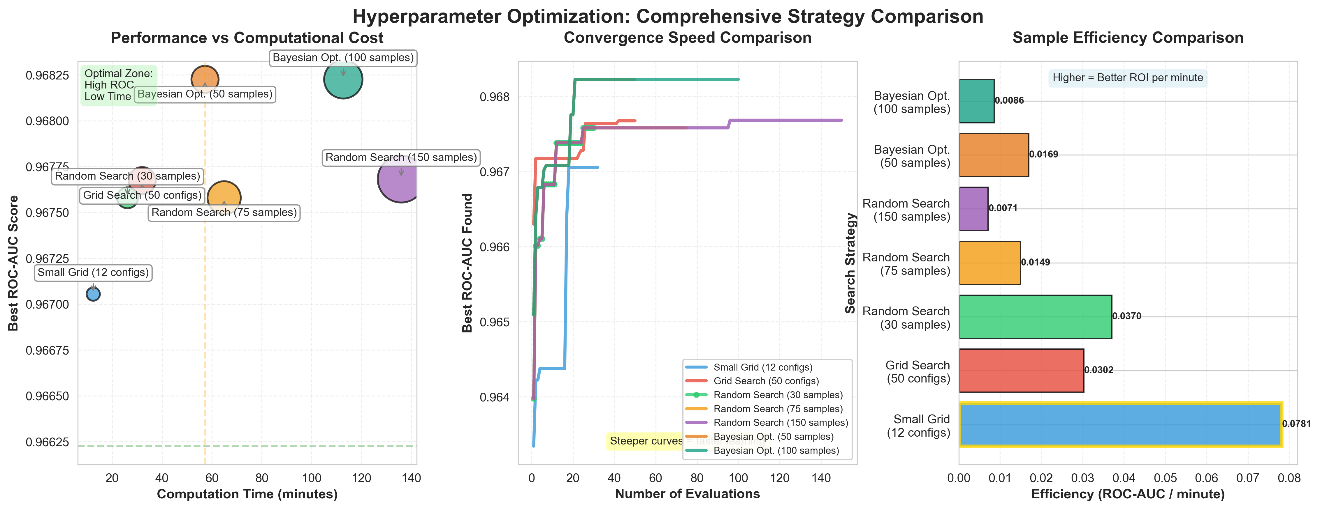
Key observations from this comparison:
- Curse of dimensionality: Grid search samples only 50 from 1,152 possible configurations (4.3% coverage), yet still requires substantial computation time
- Bayesian efficiency: Bayesian optimization with 50 iterations achieves the highest ROC-AUC (0.9682) while using less time than Random Search with 150 iterations
- Diminishing returns: Random Search shows minimal improvement from 75 to 150 iterations (+0.0001 ROC-AUC), demonstrating when additional sampling provides little benefit
- Convergence speed: The middle panel’s convergence curves reveal that Bayesian methods find good configurations faster (steeper initial curves) than random exploration
- Sample efficiency: The right panel shows Bayesian Optimization (50 samples) provides the best return on computational investment when time is limited
This real-world comparison validates the theoretical advantages discussed above: adaptive methods like Bayesian optimization outperform exhaustive grid search and pure random exploration when computational budgets are constrained.
Designing Search Spaces
The search space defines which hyperparameters to tune and what values they can take. Poor search space design wastes computational resources on irrelevant parameters or searches in the wrong regions. How do you know which hyperparameters matter enough to tune?
Start by identifying parameters with known impact. For random forests, n_estimators, max_features, and max_depth affect performance substantially. For gradient boosting, learning_rate, n_estimators, and max_depth matter most. For neural networks, learning rate, batch size, and architecture choices dominate. Regularization parameters (L1, L2 penalties) matter when overfitting occurs. Feature preprocessing choices matter when features have vastly different scales.
Scaling determines how values distribute across the range. Use log scale for hyperparameters that span orders of magnitude. Learning rates typically range from 0.0001 to 0.1, so search log-uniformly. Regularization strengths often span 0.001 to 100, requiring log scale. Tree depths and batch sizes use linear scale because they represent counts. The distinction matters: random search on a linear scale from 0.0001 to 0.1 samples mostly from 0.05 to 0.1, while log scale samples evenly across all magnitudes.
from scipy.stats import loguniform, randint
from sklearn.model_selection import RandomizedSearchCV
from sklearn.ensemble import RandomForestClassifier

# Define search space with appropriate scaling
param_distributions = {
    'n_estimators': randint(50, 500),           # Linear scale
    'max_depth': randint(5, 50),                # Linear scale
    'min_samples_split': randint(2, 20),        # Linear scale
    'max_features': ['sqrt', 'log2', 0.3, 0.5], # Categorical + continuous
    'class_weight': ['balanced', None]          # Categorical
}

# Random search with 100 iterations
random_search = RandomizedSearchCV(
    RandomForestClassifier(random_state=42),
    param_distributions=param_distributions,
    n_iter=100,
    cv=5,
    scoring='roc_auc',
    n_jobs=-1,
    random_state=42
)
Set ranges wide enough to include optimal values but narrow enough to avoid wasting evaluations on clearly poor regions. For learning rates, 0.0001 to 0.1 covers most useful values. For tree depth, 3 to 30 captures the range from simple to complex trees. Going beyond these ranges rarely helps and dilutes the search density in useful regions.
Conditional hyperparameters only matter when other parameters take certain values. Neural network dropout rate only matters when dropout layers exist. Kernel parameters for support vector machines only matter when using that kernel. Advanced search tools handle these dependencies, but simpler methods require manual structuring. Run an initial search over primary parameters, then search conditional parameters given the best primary values.
Computational Efficiency Strategies
Hyperparameter search consumes substantial computational resources. A single random forest with 500 trees on 100,000 observations takes 2 minutes to train. Evaluating 200 configurations requires 400 minutes (6.7 hours) of serial computation. Efficiency techniques reduce this burden without sacrificing search quality.
Parallel processing evaluates multiple configurations simultaneously. Random search and grid search parallelize trivially because configurations are independent. Train configuration 1 on core 1, configuration 2 on core 2, and so on. With 10 cores, 200 configurations complete in 40 minutes instead of 400. Most frameworks support this through simple parameter settings (n_jobs=-1 in scikit-learn).
But what about Bayesian optimization? Bayesian optimization parallelizes less naturally because each evaluation informs the next. Batch Bayesian optimization selects multiple configurations per iteration by modeling the joint acquisition function, but this adds complexity. For quick iterations, random search often proves more practical than parallel Bayesian optimization.
Early stopping terminates training when performance stops improving. For iterative algorithms like gradient boosting or neural networks, monitor validation error every few iterations. Stop training when error increases for 10 consecutive iterations. This prevents wasting computation on configurations that already show poor performance. Successive halving and Hyperband formalize this intuition into rigorous adaptive allocation strategies.
Coarse-to-fine search conducts broad exploration with random search, then refines promising regions with grid search or Bayesian optimization. Run 100 random samples initially. Identify the top 5 configurations. Define a narrower search space around those configurations and run another 50 evaluations. This two-phase approach balances exploration with precision.
Cheaper proxies approximate full training at lower cost. Train on a 20% data subset for initial screening. Use fewer cross-validation folds (3 instead of 10) for preliminary evaluations. For neural networks, train for 10 epochs instead of 100. These proxies sacrifice accuracy for speed during exploration, then evaluate top configurations with full resources.
Practical Tuning Workflow
Effective hyperparameter optimization follows a phased approach that progresses from broad exploration to focused refinement. This workflow balances thorough searching against computational constraints while preventing overfitting to the validation set.
Phase 1: Exploratory search with random sampling. Run 50-100 random configurations to understand the landscape. Use 3-fold cross-validation to reduce evaluation time per configuration. Record all results in a tracking system (CSV file, database, or specialized tool). Visualize hyperparameter vs performance relationships using scatter plots or parallel coordinates. This phase identifies which hyperparameters matter and where approximately optimal values lie.
Example: Fraud detection exploratory search. A fraud detection model with 8 hyperparameters undergoes exploratory random search with 80 configurations. The results show max_depth values above 15 all perform similarly (suggesting depth matters less beyond that threshold), while learning_rate below 0.01 consistently underperforms. min_samples_split between 10-20 achieves the best balance. This exploration narrows the search space for Phase 2.
Phase 2: Focused search with adaptive methods. Use Phase 1 insights to define a narrower search space. Use Bayesian optimization or Hyperband to efficiently explore this refined region. Increase cross-validation to 5 folds for more stable estimates. Run 30-50 additional evaluations. The adaptive methods concentrate effort on promising configurations while still exploring alternatives.
Phase 3: Final validation and testing. Select the top 3-5 configurations from Phase 2. Evaluate each with 10-fold cross-validation or on a separate validation set not used during tuning. Choose the configuration with the best validation performance. Test this final model on a held-out test set that was never exposed during any tuning phase. This provides an unbiased estimate of model performance on new data.
Document the entire search history. Record which hyperparameters were tuned, what ranges were explored, how many configurations were evaluated, and what computational budget was consumed. This documentation helps future tuning efforts and prevents redundant searches.
Know when to stop searching. If 20 consecutive evaluations fail to improve over the current best by more than 1%, you have likely found a near-optimal configuration. If your validation score approaches theoretical limits for the problem, further tuning provides diminishing returns. If you reach your computational budget, select the best configuration found so far.
Interpreting Optimization Results
Understanding which hyperparameters matter most helps focus future efforts and reveals insights about the learning problem. Hyperparameter importance quantifies each parameter’s impact on performance variation. How do you measure this importance systematically? Calculate importance by measuring how much validation score changes when each hyperparameter varies while others remain fixed (this isolates each parameter’s individual effect).
Visualize importance through functional ANOVA or permutation importance methods. Train models with one hyperparameter varied and others fixed at their best values. The hyperparameter that produces the largest performance range has the highest importance. For random forests, max_features typically shows high importance because it directly controls tree diversity. For boosting, learning_rate and n_estimators interact strongly and both show high importance.
Interaction effects occur when the optimal value of one hyperparameter depends on another’s value. In gradient boosting, high learning rates require fewer trees (n_estimators) while low learning rates need many trees. These parameters interact and must be tuned jointly. Visualize interactions using heat maps that show validation performance across pairs of hyperparameters.
Sensitivity analysis determines how much performance degrades when using near-optimal hyperparameters instead of optimal ones. If a hyperparameter shows low sensitivity (performance changes little when deviating from optimal), you can use simpler or faster values without sacrificing much accuracy. If it shows high sensitivity, precise tuning matters.
Overfitting to the validation set occurs when you evaluate too many configurations and select the one that happens to perform best by chance. Use nested cross-validation to get honest performance estimates. Reserve a final test set that is never exposed during hyperparameter tuning. Report both validation performance (used for selection) and test performance (unbiased estimate). Large discrepancies between these suggest overfitting the tuning process itself.
Common Pitfalls and Solutions
Search space too narrow. You define learning rates from 0.01 to 0.05, but the optimal value is 0.001. Your search finds 0.01 as “best” but misses the truly optimal region. Solution: start with wide ranges during exploratory search. If best configurations cluster at range boundaries, extend the range and search again.
Not using enough random search iterations. With 8 hyperparameters and only 20 random samples, you barely scratch the search space. Solution: use at least 10 samples per hyperparameter dimension as a rule of thumb. For 8 hyperparameters, try 80-100 random configurations before switching to adaptive methods.
Ignoring log scale for multiplicative parameters. Searching learning rates linearly from 0.0001 to 0.1 concentrates 90% of samples above 0.09. Solution: use log-uniform distributions for parameters that span orders of magnitude. This ensures equal sampling density across all scales.
Overfitting through repeated validation. You evaluate 500 configurations on the same validation set and select the best. The selected configuration performs 5% better on validation than on the final test set. Solution: use nested cross-validation where the outer loop provides unbiased estimates. Limit how many times you peek at the validation set.
Tuning parameters that don’t matter. You spend hours tuning min_samples_leaf for a random forest that already uses 1000 trees with plenty of data, gaining 0.1% accuracy. Solution: focus on high-impact parameters first. Use domain knowledge and literature to identify which parameters typically matter most for your algorithm.
Testing on the held-out set multiple times. You tune hyperparameters, test on the test set, then tune more and test again. Each test leaks information. Solution: touch the test set exactly once at the very end. Use validation sets or cross-validation for all intermediate decisions.
Ensemble-Specific Tuning Considerations
Random forests and gradient boosting machines dominate practical applications but require different tuning approaches. Random forests benefit from large n_estimators (more trees almost always helps) and carefully chosen max_features. Start with defaults (sqrt(p) for classification, p/3 for regression) and only adjust if initial results underperform. Tree depth can usually remain unrestricted because averaging controls overfitting.
Gradient boosting exhibits a fundamental tradeoff between learning_rate and n_estimators. Low learning rates (0.01) require many trees (1000+) but often achieve better performance. High learning rates (0.1) converge faster with fewer trees but may overfit. The product of these parameters determines total model capacity:
Total Capacity = learning_rate × n_estimators
Where: - learning_rate = step size for each tree’s contribution (typically 0.01-0.3) - n_estimators = number of boosting iterations (typically 100-1000) - Total Capacity = overall model complexity and learning potential
Use early stopping with a validation set to find the right n_estimators for each learning_rate.
For XGBoost specifically, tune learning_rate and n_estimators together, then adjust max_depth and min_child_weight to control tree complexity, and finally tune subsample and colsample_bytree to add randomization. This staged approach prevents wasting effort on dependent hyperparameters.
# XGBoost hyperparameter tuning workflow
import xgboost as xgb
from sklearn.model_selection import RandomizedSearchCV

# Stage 1: Learning rate and n_estimators
param_dist_stage1 = {
    'learning_rate': loguniform(0.01, 0.3),
    'n_estimators': randint(100, 1000),
    'max_depth': [6]  # Fixed
}

# Stage 2: Tree complexity (after finding best learning_rate)
param_dist_stage2 = {
    'learning_rate': [best_lr],  # Fixed from stage 1
    'n_estimators': [best_n],    # Fixed from stage 1
    'max_depth': randint(3, 10),
    'min_child_weight': randint(1, 10)
}
Bagging ensembles like random forests parallelize easily, so use all available cores (n_jobs=-1). Boosting trains sequentially, so parallelization happens at the tree level. Set nthread or n_jobs based on available resources. For large datasets, consider subsampling (use 80% of data per tree) to reduce memory and accelerate training without sacrificing much accuracy.
Integration with Course Material
The methods in this section integrate with cross-validation frameworks from Section 2 and leverage the ensemble methods from Sections 6-7. Systematic hyperparameter optimization, combined with proper validation techniques, helps your models perform well on new data, not just during development.
Design search spaces carefully. Use log scale for multiplicative parameters, set appropriate ranges, and focus on high-impact hyperparameters. Build a phased workflow that explores broadly first, then refines promising regions. Document your search history and know when to stop searching.
Interpret results to understand which hyperparameters matter and how they interact. Watch for common pitfalls like overfitting to the validation set or searching in the wrong regions. Test your final configuration on a held-out set that was never exposed during tuning.
References
Bergstra, J., & Bengio, Y. (2012). Random search for hyper-parameter optimization. Journal of Machine Learning Research, 13(1), 281-305. https://jmlr.org/papers/v13/bergstra12a.html
Li, L., Jamieson, K., DeSalvo, G., Rostamizadeh, A., & Talwalkar, A. (2018). Hyperband: A novel bandit-based approach to hyperparameter optimization. Journal of Machine Learning Research, 18(185), 1-52. https://jmlr.org/papers/v18/16-558.html
Scikit-learn developers. (2025). Tuning the hyper-parameters of an estimator. Scikit-learn documentation. https://scikit-learn.org/stable/modules/grid_search.html
© 2025 Prof. Tim Frenzel. All rights reserved. | Version 1.0.1